

Occasionally, we have the opportunity to give the database engine a helping hand, and improve the performance of a long-running SQL query. We do this, by not performing the whole query in SQL. We know better than to perform ORDER BY in SQL (see ‘Embedded SQL.doc’); now we shall see how to speed up certain types of queries.

There are three types of query which benefit from being split up, in this way:
• Any query which performs more than one full scan of a table. This inherently includes all table joins.
• Any query which features more than one logical operation in the predicate. This means any statement beginning with AND, OR and, sometimes, HAVING.
• Occasionally, where the predicate features only one operation, but where this operation is a complex one.
Consider the hypothetical query
SELECT x.a, x.b, y.a, y.d
FROM x, y
WHERE x.a = y.a
AND y.d > 42
We have joined two tables, and included a numerical comparison, as a filter for our data. The query is, of course, trivial, even if the tables contain millions of rows, but will serve as a useful template, for handling queries with more than one join, and more than one comparison, or other operation.
At the very minimum, the query will perform a full scan of either x, or y, depending on how the optimizer wants to play it, and a full scan of the index of the other table.
If there is no index on the columns we’ve selected, multiple scans of the second table will need to be performed, to find the matching data. Meanwhile, as the data is collected, each row is checked for y.d > 42.
There are two things wrong with this scenario. Firstly, all of the data is read, and re-read from the disk, which is inherently slow; secondly, the join, and the numerical comparison, are both being performed by an SQL interpreter.
So, what can be done, to make the query faster?
We are assuming, as we do with all our examples, that we have an industrial-strength machine, with at least 2GB of RAM. Given this assumption, we will simplify the query, by separating it into two subqueries, which execute as cursors, within our Pro*C, or embedded SQL program.
SELECT x.a, x.b INTO p.a, p.b
FROM x
SELECT y.a, y.d
FROM y
The first query runs to completion, giving us an array of two-element structures, in memory.
Then, the second query runs, through its cursor. As it runs, we perform two operations, which constitute the original predicate.
• We reject any rows where y.d is not greater than 42
• We check the remaining rows, one by one, against our array
of structures, for any row, where x.a = y.a. Those which
match, we keep; any which don’t, we reject.
Why is this faster than allowing the database engine to do it?
The answer is that for our trivial example, it probably isn’t. However, if we’re extracting those telephone subscribers who live in a particular area, from a table containing twenty million, and joining the result to a table of products, comprising several thousand rows, the difference in run time can be over an order of magnitude.
The key to performing searches on memory-based arrays is a set of tools, the best of which we will now examine.
Hash tables, which we consider first, are an order of magnitude faster than linear searches. However, they are not the fastest way of retrieving data from an array of structures. They carry an overhead of the time taken to actually create the table, which is approximately equal to the time taken to access each element.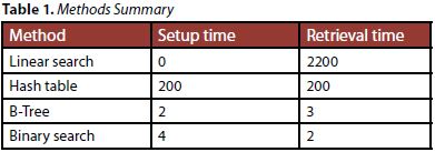
A similar disadvantage is shared by the binary tree, or B-tree, described below, which needs time to create the tree, whereas the binary search, or ‘divide and conquer’ algorithm, requires its input data to be sorted in ascending order.
The difference is that b-trees and binary searches are two orders of magnitude faster than hash tables.
The following summary lists all four methods, applied to retrieving all 2 million elements from an array of 2 million such elements. The data was originally extracted from a database table, a single scan of which took 87 seconds. This indicates that it would have taken a prohibitively long time to individually extract each of the 2 million rows.
Hash Tables
Simplistically speaking, a hash table is a random access matrix of variables and values, where the variables are also the index into the matrix of values.
Instead of saying ‘for(I = 0; I < 1000; I++)….’, and waiting for the sought after value to fly by, we can simply ask the hash table for the value corresponding to the given variable. Unix has four hash table manipulation
functions:
hcreate(length)
allocates space for a hash table, of size ‘length’ elements.
hsearch(key, ENTER)
Makes a hash table entry, for variable ‘key’
hsearch(key, FIND)
Retrieves an entry described by ‘key’, from the hash table.
hdestroy(void)
Deletes a hash table. The data type of ‘key’ is defined by the typedef ENTRY, in <search.h>, which must be included, if we want to use the hash table functions.
struct entry {
char *key;
char *data;
};
Since hash tables can be used with arrays of complex data structures, the pointers to char are an indication of how the hash table is implemented.
A hash table only stores hash values, and pointers to the original data. This data must persist, with unchanged keys and addresses, throughout the life of the table.
The data itself can change, and the pointer will still correctly retrieve it, but its address must be constant.
For obvious reasons, the key must be unique, so the same criteria must be applied to its choice as are applied to choosing the primary key to a database table. If the target array comprises the rows of a table, which has been extracted into memory, the primary key of the table is an obvious choice.
There is one restriction on the choice of a key. The hash table comparison function is strcmp(), which means that the key has to be an ASCII string, and numbers have to be represented by their ASCII values.
However, the overhead of the extra sprintf() is negligible, compared with the saving of time, especially when scanning a huge array.
By way of example, suppose that we have an array of 1000 data structures, each of which describes a product, as per:
struct product {
char product_code[10];
char colour[25];
float length;
int style;
float price;
};
struct product products[1000];
ENTRY hhash;
Early in our code, we create the 1000 element hash table, like this:
if(hcreate(1000) == 0){
printf(“Can’t allocate memory for hash tablen”);
exit(-1);
}
As we create or load the array of product structures, we add an extra step, to make the hash table entries:
for(I = 0; I < 1000; I++){
get_product_data(products[I]);
hhash.key = (void *)products[I].product_code;
hhash.data = (void *)&products[I];
if(hsearch(hhash, ENTER) == NULL){
printf(“Hash table fulln”);
}
/* do other stuff… */
}
Some time later, we are doing some processing in another loop, and need to find the colour, corresponding to a product code:
char * pc;
struct product temp;
for(j = 0; j < 20000000; j++){
/*
* process a lot of customer data
*/
pc = customer_products[j].product_code;
/* Now, we need the colour */
hhash.key = (void *)pc
if((temp = hsearch(hentry, FIND)) == NULL) {
printf(“No such entryn”);
} else {
strcpy(customer_products[I].colour, ((struct
product *)temp->data)->colour).
}
}
The linear search alternative to using a hash table would have been an inner loop, making up to 1000 iterations, for every iteration of the outer loop.
Binary Trees, or B-Trees
The binary tree is used extensively within many databases, for the creation of indices. Creation of binary trees represents an extremely small overhead, and they are second only to the binary search in terms of data access time, but they provide the added advantage, that nodes can be deleted, and elements of the tree can be modified, while traversing it from a given starting point. The binary search, on the other hand, is just that: a search.
Unix provides a set of binary tree creation and search routines, which have the following functionality:
tsearch() Adds a node to the b-tree
tfind() Searches the b-tree for a given node
tdelete() Deletes a node from the tree
twalk() Traverses the tree, and performs a userspecified
action at each node.
To support these activities, we need to supply a comparison routine, identical to the type used by qsort().
As with qsort(), it needs to take two arguments, which are the nodes to compare, and needs to return –1, 0 or +1, depending on whether the nodes are equal or not. See “Embedded SQL.doc” for code samples. Syntax for tsearch is:
void *tsearch(void *key, void **root, int (*cmp)(void *,void *));
The ‘key’ parameter is a pointer to the element of the structure, by which we will later want to search the tree.
The rather ugly **root, is a pointer to a variable, which will contain the address of the root of the tree, when we have one. For the moment, we need to point it at an address of NULL, so we need the following clumsy acrobatics:
struct product *xroot;
struct product **root;
xroot = NULL; /* this will get set to the root of
the new tree */
*root = xroot; /* this must point to it */
Taking the earlier example, using struct product, we would create our b-tree, like this:
for(i = 0; i < 1000; i++){
if(tsearch((void *)products[i].product_code, (void
**)root, cmpfn) == NULL){
printf(“Error creating binary treen”);
break;
}
}
The syntax of the tfind() command is identical, except that we don’t force a NULL into the address of the root of the tree.
void *tfind(void *key, void **root, int (*cmp)(void *,void *));
Taking the same example as for the hash table, let’s assume that, some time later, we are doing some processing in another loop, and need to find the colour, corresponding to a product code:
char * pc;
struct product temp;
for(j = 0; j < 20000000; j++){
/*
* process a lot of customer data
*/
pc = products[j].product_code);
/* Now, we need the colour */
if(tfind((void *)pc, (void **)root, cmpfn) != NULL){
printf(“Colour >%s< found in treen”,
products[i].colour);
}
}
Note that we don’t need to perform a loop in order to find our colour.
If we need to delete a particular node, we invoke the tdelete() function, with the same syntax as for the preceding commands:
void *tfind(void *key, void **root, int (*cmp)(void *,void *));
Let ‘I’ be the index of the array element we wish to delete,
then:
if(tdelete((void *)products[I].product_code,
(void **)root, cmpfn) != NULL){printf(“Deleted >%s< from treen”,
products[i].product_code);
}
Let us assume that, as part of our data manipulation, we need to update the data in our structures. Perhaps we need to decrease the price for all pink items, because there is a weekend sale.
To perform the equivalent of a global edit, on all the members of the array, individually, would take an extremely long time if, as in real life, the array contained more than the trivial number of items shown above. Worse, if this array had to be processed for every store in the country, inside another loop, the run time would be prohibitive.
This is where we would use twalk(), which has a syntax as per:
void twalk(void *root, void(*action) (void *, VISIT, int));
The parameter ‘root’ points to the starting node which, in theory, can be any node. However, the traversal is limited to all nodes below this root so, if we wish to visit all nodes, we need to set the root to the first item loaded into our tree, i.e products[0].
The ‘action’ parameter is a function, which we need to write, to tell twalk() what it should do, as it accesses each node. As each node is accessed, twalk() will pass to our function, three arguments, of types void *, VISIT, and int.
The first argument is a pointer to the node currently being visited, the second is an enumerated data type, whose values are as follows:
0: preorder. The node is visited before any of its children.
1: postorder. Node is visited after its left child and before its right
2: endorder. The node is visited after both children
3: leaf. This node is a leaf
Basically, preorder means that this is the first time the node has been visited, postorder means the second time, and endorder means the third time.
Leaf means that this node is a leaf of the tree.
The last argument is the level of the node, relative to the root of the tree, which is level zero.
From these parameters, our function can deduce where we are and what data we’re looking at, and perform appropriate actions.
If we had defined a function modify_data(), to perform our manipulation, then we would call twalk() thus:
twalk(root, modify_data);
Binary Search
When all we want to do, is find data fast, we use the binary search, which is the fastest of all of the non-linear search techniques. It uses the familiar ‘divide and conquer’ algorithm, similar to the one used by qsort() to sort data.
Before running bsearch(), the data must be sorted, using qsort(). There is only one function call to remember,
bsearch(void *key, void *base, size_t numelmt, size_t elmt_size, int (*cmp)(void *, void *));
As before, cmp() is the usual comparison function, and key is the item for which we are searching. The parameter numelmt, is the length of our array, and elmt_size is sizeof (our data structure). It is called, quite simply, as:
char *pc;
struct product *pp;
pc = products[i].product_code;
if((pp = bsearch((void *)pc, product, 1000,
sizeof(struct product), cmp)) != NULL){
printf(“Product >%s< found in arrayn”,
pp->product_code);
}
Mark Sitkowski
Mark is a Chartered Engineer, and a Corporate Member of the Institution of Electrical Engineers in London. His early career revolved around the writing of analog and digital circuit simulators and digital signal processing applications. In Australia, he moved to writing financial software for the major banks, and telecommunications software for telcos, together with conducting training courses on Unix and database applications. He is currently a consultant to Forticom Security, having written an application for an uncrackable user authentication system.
Design Simulation Systems Ltd: http://www.designsim.com.au | Consultant to Forticom Security: http://www.forticom.com.au | xmarks@exemail.com.au
")
")